LEFTIST
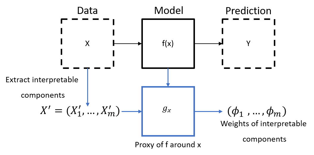
Agnostic Local Explanation for Time Series Classification (LEFTIST) by Guilleme et al. (2019) [1] adapted LIME for time series classification and proposed to use prefixed (both the length and the position) shapelets as the interpretable components and provide the feature importance of each shapelet.

The code in TSInterpret is based on the authors implementation . The image is reproduced from [1].
[1] Guillemé, Maël, et al. "Agnostic local explanation for time series classification." 2019 IEEE 31st International Conference on Tools with Artificial Intelligence (ICTAI). IEEE, 2019.
import os
os.environ['TF_CPP_MIN_LOG_LEVEL'] = '3'
import pickle
import numpy as np
import torch
from ClassificationModels.CNN_T import ResNetBaseline, UCRDataset
from tslearn.datasets import UCR_UEA_datasets
import sklearn
Dataset
dataset='GunPoint'
Load Data
Load Data and reshape the data to fit a 1D-Conv ResNet. Note that the input for a 1D-Conv Resnet hat the shape (batch, features, timesteps).
train_x,train_y, test_x, test_y=UCR_UEA_datasets().load_dataset(dataset)
train_x = train_x.reshape(-1,1,  train_x.shape[-2])
test_x = test_x.reshape(-1,1,  test_x.shape[-2])
enc1=sklearn.preprocessing.OneHotEncoder(sparse=False).fit(np.vstack((train_y.reshape(-1,1),test_y.reshape(-1,1))))
pickle.dump(enc1,open(f'../../ClassificationModels/models/{dataset}/OneHotEncoder.pkl','wb'))

train_y=enc1.transform(train_y.reshape(-1,1))
test_y=enc1.transform(test_y.reshape(-1,1))
/home/jacqueline/.local/share/virtualenvs/TSInterpret-NXJYnQDU/lib/python3.10/site-packages/sklearn/preprocessing/_encoders.py:972: FutureWarning: `sparse` was renamed to `sparse_output` in version 1.2 and will be removed in 1.4. `sparse_output` is ignored unless you leave `sparse` to its default value.
  warnings.warn(
Model Training
Loads a pretrained 1D-Conv ResNet.
n_pred_classes =train_y.shape[1]
train_dataset = UCRDataset(train_x.astype(np.float64),train_y.astype(np.int64))
test_dataset = UCRDataset(test_x.astype(np.float64),test_y.astype(np.int64))
train_loader = torch.utils.data.DataLoader(train_dataset,batch_size=16,shuffle=True)
test_loader = torch.utils.data.DataLoader(test_dataset,batch_size=1,shuffle=False)
model = ResNetBaseline(in_channels=1, num_pred_classes=n_pred_classes)
model.load_state_dict(torch.load(f'../../ClassificationModels/models/{dataset}/ResNet'))
<All keys matched successfully>
Interpretability Algorithm
Using a interpretability algorithm consists of 4 steps:
1. Load the Interpretability Method
2. Instaniate the Method with the desired Parameters
3. Call the explain Method
4. Plot the results
2. Initialization
LEFTIST works on all type of black-box classificators and can therefore be used with PyTorch (PYT), TensorFlow (TF), Sklearn (SK) and predict function, as long as the predict function returns a probability distribution. The Initialization takes the following arguments:
model_to_explain: The model to be explaines.data: Reference Set of type (X_train, y_train).mode: Second dimension 'time' or 'feat'.backend: TF, PYT, SK or func.transform_name: Name of transformer.* `uniform`: Mean Transform * `straight_line`: StraightlineTransform * `background`: RandBackgroundTransform
learning_process_name: 'Lime' or 'Shap'.nb_interpretable_feature: number of desired features.
model.eval()
explained_instance = train_x[0]
label=train_y[0]
nb_interpretable_feature = 10
explanation_size = 1
nb_neighbors = 1000
learning_process_name = 'Lime'
transform_name = 'background'
model_to_explain=model
from TSInterpret.InterpretabilityModels.leftist.leftist import LEFTIST
/home/jacqueline/.local/share/virtualenvs/TSInterpret-NXJYnQDU/lib/python3.10/site-packages/tqdm/auto.py:21: TqdmWarning: IProgress not found. Please update jupyter and ipywidgets. See https://ipywidgets.readthedocs.io/en/stable/user_install.html
  from .autonotebook import tqdm as notebook_tqdm
leftist = LEFTIST(model_to_explain,(test_x,test_y),mode='feat', backend='PYT', \
learning_process_name='Lime',transform_name=transform_name, explanation_size=explanation_size,nb_neighbors=1000)
label=np.argmax(label)
3. Call the explain method.
Prepare the instance and the predicted label of the instance as parameters for the explain methods.
model_to_explain: The model to be explaines.nb_neighbors: Number if neighbors used in the calculatuions.idx_label: index of label to explain. If None, return an explanation for each label.explanation_size: Size of desired explanation.
explanations = leftist.explain(np.array(explained_instance),label)
4. Visualize
Visualize the explanation by calling .plot(). Parameters are the original instance to be explained and the explanation.
leftist.plot(np.array([explained_instance]),np.array([explanations[0]]))
feat
NOT Time mode
-1
1
0
Additional Examples, e.g. for the use with LSTM or TF can be found here.